44 how to put data labels in excel chart

How to Use Excel Pivot Table Label Filters In an Excel pivot table, you might want to hide one or more of the items in a Row field or Column field. To do that, you could click the drop down arrow for the Row or Column Labels, then remove the check mark for items you want to remove. For example, to hide the data for 7-Feb-10, you'd click on the check mark to remove it. How to: Display and Format Data Labels - DevExpress Add Data Labels to the Chart Specify the Position of Data Labels Apply Number Format to Data Labels Create a Custom Label Entry After you create a chart, you can add a data label to each data point in the chart to identify its actual value. By default, data labels are linked to data that the chart uses.

How to Create a Run Chart in Excel (2021 Guide) | 2 Free Templates In the Format Data Series task pane, switch to the Fill & Line tab. Click " Marker. " Select " Marker Options ." In the " Type " dropdown menu, customize your marker type. Set the " Size " value to " 8 ." Add Custom Data Labels You can make your time series plot more informative by adding data labels reflecting the actual values.

How to put data labels in excel chart

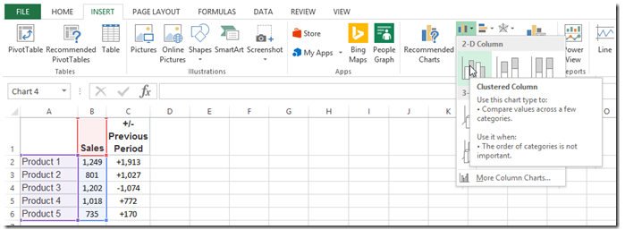
How to Change the X-Axis in Excel - Alphr Follow the instructions to change the text-based X-axis intervals: Open the Excel file and select your graph. Now, right-click on the Horizontal Axis and choose Format Axis… from the menu. Select... How To Show Two Sets of Data on One Graph in Excel in 8 Steps To do so, click and drag your mouse across all the data you want, including the names of the columns and rows. You can check that you selected the data by looking for the cells to be gray instead of white. 3. Click the "Insert" tab and then look at the "Recommended Charts" in the charts group How to make a line graph in excel with multiple lines It's easy to make a line chart in Excel. Follow these steps: 1 Select the data range for which we will make a line graph. 2 On the Insert tab, Charts group, click Line and select Line with Markers. Quickly Change Diagram Views A quick way to change the appearance of a graph is to use Chart Styles , Quick Layout, and Change Colors.

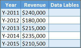
How to put data labels in excel chart. How to Make a Pie Chart in Excel & Add Rich Data Labels to The Chart! Creating and formatting the Pie Chart. 1) Select the data. 2) Go to Insert> Charts> click on the drop-down arrow next to Pie Chart and under 2-D Pie, select the Pie Chart, shown below. 3) Chang the chart title to Breakdown of Errors Made During the Match, by clicking on it and typing the new title. 4) With the chart title still selected, go to ... How do I add labels to Gantt Chart? - Microsoft Power BI Community You can create a measure like this one that has both values and then use that as your data label. DataLabel = MIN (Sheet1 [Leaving Date]) & " - " & MIN (Sheet1 [Returning Date]) Pat Did I answer your question? Mark my post as a solution! Kudos are also appreciated! To learn more about Power BI, follow me on Twitter or subscribe on YouTube. How to: Display and Format Data Labels - DevExpress When data changes, information in the data labels is updated automatically. If required, you can also display custom information in a label. Select the action you wish to perform. Add Data Labels to the Chart. Specify the Position of Data Labels. Apply Number Format to Data Labels. Create a Custom Label Entry. Excel: How to Create a Bubble Chart with Labels - Statology Then click OK and in the Format Data Labels panel on the right side of the screen, uncheck the box next to Y Value and choose Center as Label Position. The following labels will automatically be added to the bubble chart: Step 4: Customize the Bubble Chart. Lastly, feel free to click on individual elements of the chart to add a title, add axis ...

chandoo.org › wp › change-data-labels-in-chartsHow to Change Excel Chart Data Labels to Custom Values? May 05, 2010 · Now, click on any data label. This will select “all” data labels. Now click once again. At this point excel will select only one data label. Go to Formula bar, press = and point to the cell where the data label for that chart data point is defined. Repeat the process for all other data labels, one after another. See the screencast. Custom Chart Data Labels In Excel With Formulas Follow the steps below to create the custom data labels. Select the chart label you want to change. In the formula-bar hit = (equals), select the cell reference containing your chart label's data. In this case, the first label is in cell E2. Finally, repeat for all your chart laebls. Excel: How To Convert Data Into A Chart/Graph - Digital Scholarship ... 7: To add axis titles, data labels, legend, trendline, and more, click the graph you just created. A new tab titled "Chart design" should appear. In the upper menu of that tab, you should see a section called "add chart element." 8: In "add chart element," you can customize your graph to your liking . STEP 9: Don't forget to save your work! › 509290 › how-to-use-cell-valuesHow to Use Cell Values for Excel Chart Labels Mar 12, 2020 · Select the chart, choose the “Chart Elements” option, click the “Data Labels” arrow, and then “More Options.” Uncheck the “Value” box and check the “Value From Cells” box. Select cells C2:C6 to use for the data label range and then click the “OK” button.

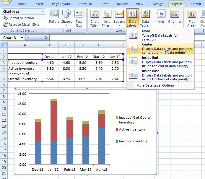
How to Show Percentages in Stacked Column Chart in Excel? Step 3: To create a column chart in excel for your data table. Go to "Insert" >> "Column or Bar Chart" >> Select Stacked Column Chart . Step 4: Add Data labels to the chart. Goto "Chart Design" >> "Add Chart Element" >> "Data Labels" >> "Center". You can see all your chart data are in Columns stacked bar. Data label in the graph not showing percentage option. only value ... Data label in the graph not showing percentage option. only value coming Team, Normally when you put a data label onto a graph, it gives you the option to insert values as numbers or percentages. In the current graph, which I am developing, the percentage option not showing. Enclosed is the screenshot. Display data point labels outside a pie chart in a paginated report ... Create a pie chart and display the data labels. Open the Properties pane. On the design surface, click on the pie itself to display the Category properties in the Properties pane. Expand the CustomAttributes node. A list of attributes for the pie chart is displayed. Set the PieLabelStyle property to Outside. Set the PieLineColor property to Black. How to Create and Customize a Treemap Chart in Microsoft Excel Either right-click the chart and pick "Format Chart Area" or double-click the chart to open the sidebar. On Windows, you'll see two handy buttons on the right of your chart when you select it. With these, you can add, remove, and reposition Chart Elements. And you can pick a style or color scheme with the Chart Styles button.

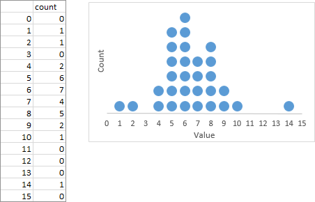
Make Technical Dot Plots in Excel | LaptrinhX

Format Chart Axis in Excel - Axis Options Formatting a Chart Axis in Excel includes many options like Maximum / Minimum Bounds, Major / Minor units, Display units, Tick Marks, Labels, Numerical Format of the axis values, Axis value/text direction, and more. However, there are a lot more formatting options for the chart axis, in this blog, we will be working with the axis options and ...

How To Use Dynamic Data Labels To Create Interactive Excel Charts

stackoverflow.com › questions › 48559387stacked column chart for two data sets - Excel - Stack Overflow Feb 01, 2018 · After I stored my data correctly I can make my chart with a javascript library, I used Highcharts (pretty similar to google charts), it has a good documentation with lots of examples. I put all the data and some few options in a series variable which uses the format of highcharts, like so:

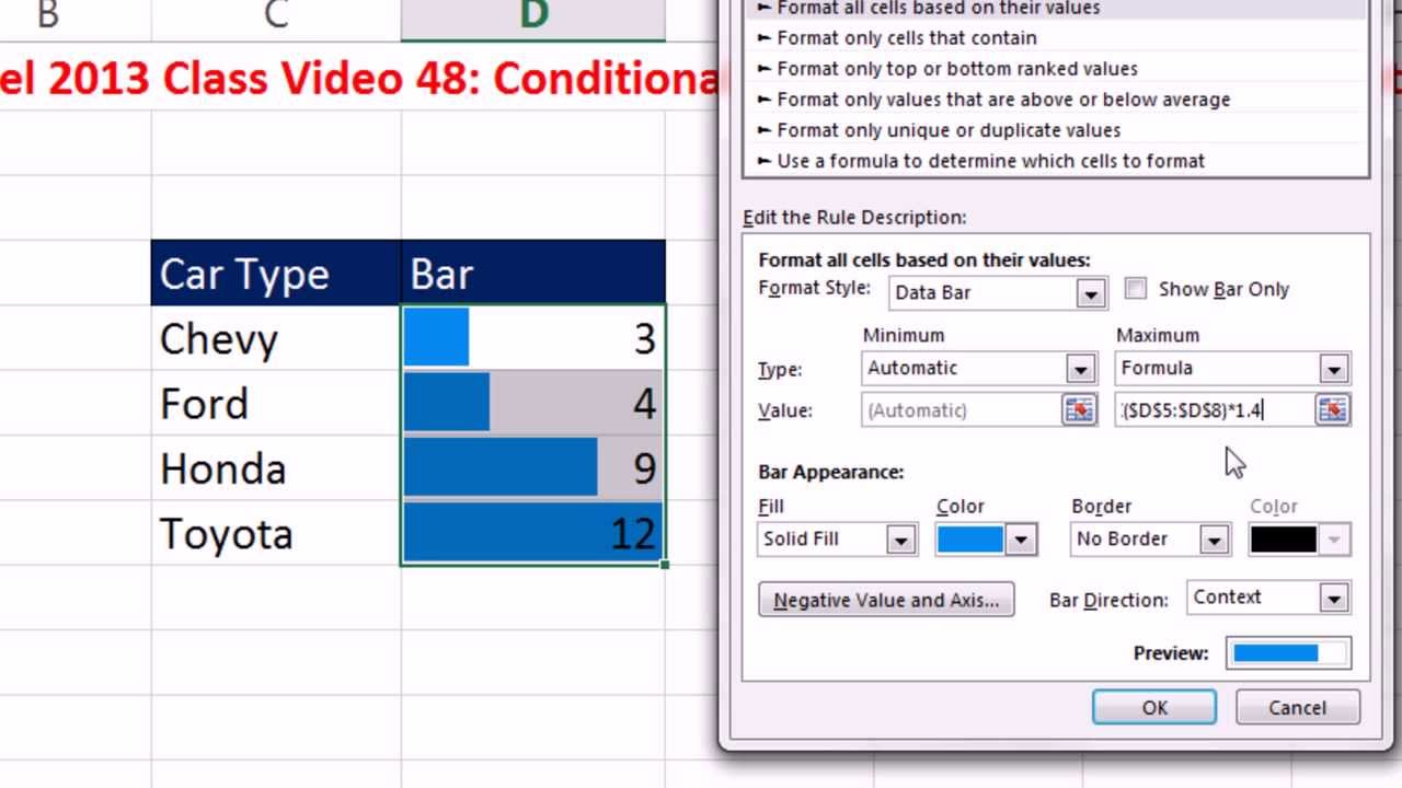
Highline Excel 2013 Class Video 48: Conditional Formatting: Bar Chart with Data Labels - YouTube

How to Make a Scatter Plot in Excel and Present Your Data Add Labels to Scatter Plot Excel Data Points. You can label the data points in the X and Y chart in Microsoft Excel by following these steps: Click on any blank space of the chart and then select the Chart Elements (looks like a plus icon). Then select the Data Labels and click on the black arrow to open More Options. Now, click on More Options ...

How-to Use Data Labels from a Range in an Excel Chart - Excel Dashboard Templates

How to Create Multi-Category Charts in Excel? - GeeksforGeeks Step 1: Insert the data into the cells in Excel. Now select all the data by dragging and then go to "Insert" and select "Insert Column or Bar Chart". A pop-down menu having 2-D and 3-D bars will occur and select "vertical bar" from it. Select the cell -> Insert -> Chart Groups -> 2-D Column Bar Chart Insertion Multi-Category Chart

MS Excel 2010 / How to remove data labels from the chart - YouTube

How to Add Labels to Scatterplot Points in Excel - Statology Next, click anywhere on the chart until a green plus (+) sign appears in the top right corner. Then click Data Labels, then click More Options… In the Format Data Labels window that appears on the right of the screen, uncheck the box next to Y Value and check the box next to Value From Cells.

Add label to Excel chart line • AuditExcel.co.za

peltiertech.com › select-data-display-in-excelSelect Data to Display in an Excel Chart With Option Buttons Feb 17, 2015 · You could put the chart and option buttons on the active sheet, and all of the data (and the option button linked cell) can go onto another sheet, and you can hide this other sheet if you want. Or you can place the original data on the same sheet as the chart and option buttons, and the formulas onto another sheet, a hidden sheet if desired.

Format Number Options for Chart Data Labels in Excel 2011 for Mac

How to Apply a Filter to a Chart in Microsoft Excel Select the data for your chart, not the chart itself. Go to the Home tab, click the Sort & Filter drop-down arrow in the ribbon, and choose "Filter." Click the arrow at the top of the column for the chart data you want to filter. Use the Filter section of the pop-up box to filter by color, condition, or value. Advertisement

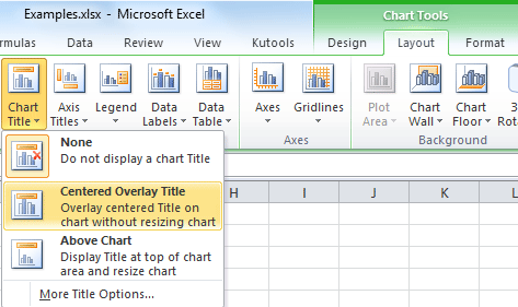
How to add a chart title in Excel?

Prevent Overlapping Data Labels in Excel Charts - Peltier Tech Apply Data Labels to Charts on Active Sheet, and Correct Overlaps Can be called using Alt+F8 ApplySlopeChartDataLabelsToChart (cht As Chart) Apply Data Labels to Chart cht Called by other code, e.g., ApplySlopeChartDataLabelsToActiveChart FixTheseLabels (cht As Chart, iPoint As Long, LabelPosition As XlDataLabelPosition)

Excel Dashboard Templates How-to Put Percentage Labels on Top of a Stacked Column Chart - Excel ...

How to Print Labels from Excel - Lifewire Choose Start Mail Merge > Labels . Choose the brand in the Label Vendors box and then choose the product number, which is listed on the label package. You can also select New Label if you want to enter custom label dimensions. Click OK when you are ready to proceed. Connect the Worksheet to the Labels

Making BCG Matrix in Excel - How To - PakAccountants.com

› documents › excelHow to wrap X axis labels in a chart in Excel? (1) If the chart area is still too narrow to show all wrapped labels, the labels will keep rotated and slanted. In this condition, you have to widen the chart area if you need the labels wrapping in the axis. (2) The formula ="Orange"&CHAR(10)&"BBBB" will wrap the labels in the source data too in Excel 2010.

How to create Custom Data Labels in Excel Charts – Efficiency 365

› charts › dynamic-chart-dataCreate Dynamic Chart Data Labels with Slicers - Excel Campus Feb 10, 2016 · Typically a chart will display data labels based on the underlying source data for the chart. In Excel 2013 a new feature called “Value from Cells” was introduced. This feature allows us to specify the a range that we want to use for the labels. Since our data labels will change between a currency ($) and percentage (%) formats, we need a ...

How to Create Progress Charts (Bar and Circle) in Excel - Automate Excel

How to make a scatter plot in Excel - Ablebits Tick off the Data Labels box, click the little black arrow next to it, and then click More Options… On the Format Data Labels pane, switch to the Label Options tab (the last one), and configure your data labels in this way: Select the Value From Cells box, and then select the range from which you want to pull data labels (B2:B6 in our case).

Excel Bar Charts - Clustered, Stacked - Template - Automate Excel

How to Create a Histogram in Excel: A Step-by-Step Guide This chart is available in Excel 2016 and later, so if you have an earlier version of Excel, you can follow the second method provided in this post. There are 41 scores in this data, and we want to create a histogram that distributes the scores over intervals of 10 starting from the score of 40, and ending with 100 (the maximum score).

Change Chart Data Labels : Chart Data « Chart « Microsoft Office Excel 2007 Tutorial

› custom-data-labels-in-xImprove your X Y Scatter Chart with custom data labels May 06, 2021 · Thank you for your Excel 2010 workaround for custom data labels in XY scatter charts. It basically works for me until I insert a new row in the worksheet associated with the chart. Doing so breaks the absolute references to data labels after the inserted row and Excel won't let me change the data labels to relative references.

Share :