39 conditional formatting data labels excel

Custom Data Labels with Colors and Symbols in Excel Charts - [How To] Step 4: Select the data in column C and hit Ctrl+1 to invoke format cell dialogue box. From left click custom and have your cursor in the type field and follow these steps: Press and Hold ALT key on the keyboard and on the Numpad hit 3 and 0 keys. Let go the ALT key and you will see that upward arrow is inserted. How to Strikethrough in EXCEL using Conditional Formatting? Select all the cells in which you want to remove the conditional formatting. Go to HOME TAB>CONDITIONAL FORMATTING>CLEAR RULES>CLEAR RULES FROM ENTIRE SHEET. [ Shown as 2 in the picture below.] All the STRIKETHROUGH conditional formatting will be removed i.e. All the cells containing the strikethrough data will be removed.

How to Create Excel Charts (Column or Bar) with Conditional Formatting Conditional formatting is the practice of assigning custom formatting to Excel cells—color, font, etc.—based on the specified criteria (conditions). The feature helps in analyzing data, finding statistically significant values, and identifying patterns within a given dataset.

Conditional formatting data labels excel

Conditional Formatting Shapes - Step by step Tutorial Let's see step by step how to create it: First, select an already formatted cell. In the picture below, we have created a little example of this. We will pay attention to the range D5:D6. You can see the rules in the Rules Manager window. We didn't make it overly complicated. Creating Conditional Data Labels in Excel Charts - YouTube We can make labels appear on our charts that don't have to do with the raw numbers that built the chart - and we can make them show up or not based on whatever conditions we want. In this tutorial,... How to Use Conditional Formatting Based on Date in Microsoft Excel If you want to create a quick and easy conditional formatting rule, this is a convenient way to go. Open the sheet, select the cells you want to format, and head to the Home tab. RELATED: How to Use Conditional Formatting to Find Duplicate Data in Excel. In the Styles section of the ribbon, click the drop-down arrow for Conditional Formatting.

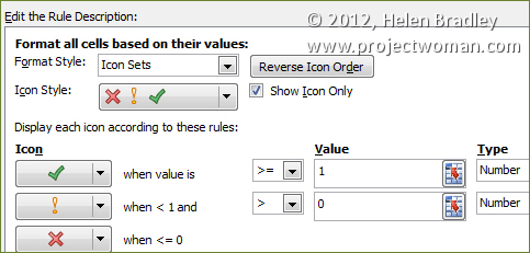
Conditional formatting data labels excel. Excel Data Analysis - Conditional Formatting Follow the steps to conditionally format cells − Select the range to be conditionally formatted. Click Conditional Formatting in the Styles group under Home tab. Click Highlight Cells Rules from the drop-down menu. Click Greater Than and specify >750. Choose green color. Click Less Than and specify < 500. Choose red color. Conditional Formatting in Excel - a Beginner's Guide Click Conditional Formatting, then select Icon Set to choose from various shapes to help label your data. For this example, let's use the arrow icon set to show whether our highlighted data, the Variance column, has increased or decreased. Now, you'll see that the data has arrow icons accompanying their values in the cells. Use conditional formatting to highlight information Conditional formatting can help make patterns and trends in your data more apparent. To use it, you create rules that determine the format of cells based on their values, such as the following monthly temperature data with cell colors tied to cell values. Change the format of data labels in a chart To get there, after adding your data labels, select the data label to format, and then click Chart Elements > Data Labels > More Options. To go to the appropriate area, click one of the four icons ( Fill & Line, Effects, Size & Properties ( Layout & Properties in Outlook or Word), or Label Options) shown here.

Conditional Formatting to Distinguish Between Labels and Numbers I want to conditionally format each cell, so that the text is yellow, the numbers are blue, and the blank cells are green. I tried by setting up a new rule under conditional formatting, then selecting "use a formula to determine which cells to format", then using some combinations of the if, istext, isnumber, etc. combinations. Please advise. Conditional format chart data labels - My Online Training Hub Lance 354 524 550 I create a bar chart that from this data, and display the data label for Actual. I would like to format this data label so that it displays in Red if the value of Actual is less than the value of On Track. Otherwise, it will just display as Blue, which is the format color right now. Excel conditional formatting Icon Sets, Data Bars and Color Scales Select all cells in column A, except for the column header, and create a conditional formatting icon set rule by clicking Conditional Formatting > Icon sets > More Rules... In the New Formatting Rule dialog, select the following options: Click the Reverse Icon Order button to change the icons' order. Select the Icon Set Only checkbox. Solved: Conditional Formatting Data Labels Solved: HI All, I have a line graph which has some values shown as data labels, i would like to conditionally format these labels. Can anyone help?

Excel Conditional Formatting - Data Bars - W3Schools Click on the Conditional Formatting icon in the ribbon, from Home menu. Select Data Bars from the drop-down menu. Select the "Green Data Bars" color option from the Gradient Fill menu. Note: Both Gradient Fill and Solid Fill work the same way. The only difference between those, and the color options are aesthetic. How to change chart axis labels' font color and size in Excel? Sometimes, you may want to change labels' font color by positive/negative/ in an axis in chart. You can get it done with conditional formatting easily as follows: 1. Right click the axis you will change labels by positive/negative/0, and select the Format Axis from right-clicking menu. 2. Format Data Labels in Excel- Instructions - TeachUcomp, Inc. To format data labels in Excel, choose the set of data labels to format. To do this, click the "Format" tab within the "Chart Tools" contextual tab in the Ribbon. Then select the data labels to format from the "Chart Elements" drop-down in the "Current Selection" button group. Then click the "Format Selection" button that ... How to do conditional formatting of a label in Excel VBA Function ConditionalFormatNumber (n As Double) As String If n > 1000000 Then ConditionalFormatNumber = Format (n / 1000000, "$#,##0.00,,""M""") ElseIf n > 1000 Then ConditionalFormatNumber = Format (n / 1000, "$#,##0.00, ""K""") Else ConditionalFormatNumber = Format (n, "$#,##0.0") End If End Function Share Improve this answer

BYS [SSV1015] – Pivot Tables | Build Your Skill

How-to Make Conditional Label Values in an Excel Stacked ... Step-by-Step · 1) After you create your Chart Data Range, you now need to create the conditional labels data range. · 2) Create your chart by highlighting cells ...

Moving X-axis labels at the bottom of the chart below negative values in Excel - PakAccountants.com

Conditional formatting for Excel column charts - Think Outside The Slide Additional formatting. The colors used for each data series is from the color theme being used for this Excel file. You can assign more meaningful colors for each data series. You can also add data labels to each series. It is a good idea to format the data label text to have the same color as the column it is representing.

MS Excel 2007 Tutorial: Thermometer Chart in Excel

Conditional Formatting of Excel Charts - Peltier Tech From the Data Label options, I am able to include any of the 4 data cateogires; however, i cannot include the customer name. ... Conditional Formatting of Excel Charts - Peltier Tech Blog […] Conditional Format Chart says: Sunday, June 26, 2016 at 4:13 pm […] document.write(''); y tutorial on this topic is at Conditional Formatting of ...

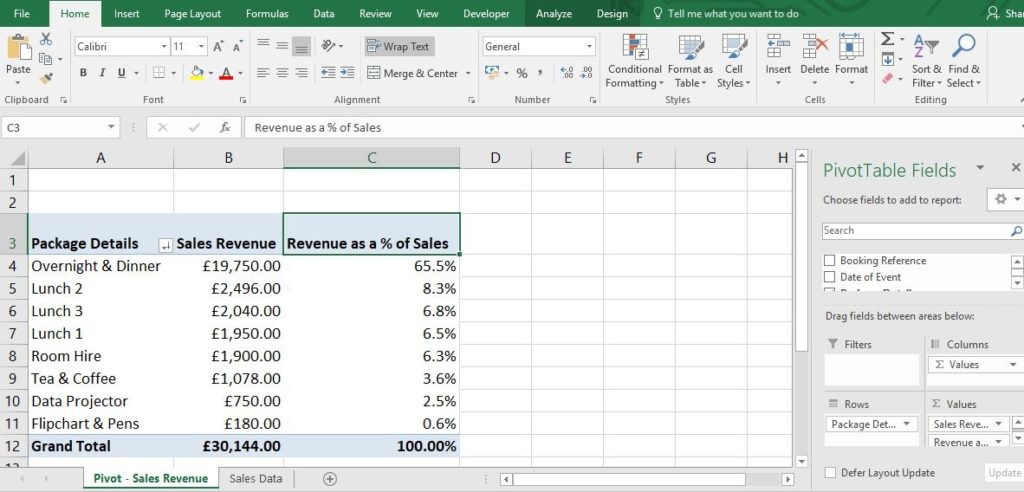
How to Create a MS Excel Pivot Table – An Introduction | SIMPLE TAX INDIA

Is it possible to conditionally format Data Labels on a dynamic ... For example, when numbers 0-3 are plotted on the dynamic chart above their data label's font colour turns red, and if numbers 7-10 are plotted these turn green.

Recording Yes, No, Maybe so in Excel « projectwoman.com

Conditional Formatting with Data Validation - Microsoft Tech Community Select the range in column C that you want to format, for example C2:C100. The first cell in the range (C2 in this example) should be the active cell in the selection. On the Home tab of the ribbon, select Conditional Formatting > New Rule... Select 'Use a formula to determine which cells to format'. Enter the formula

How to Create Multi-Category Chart in Excel - Excel Board

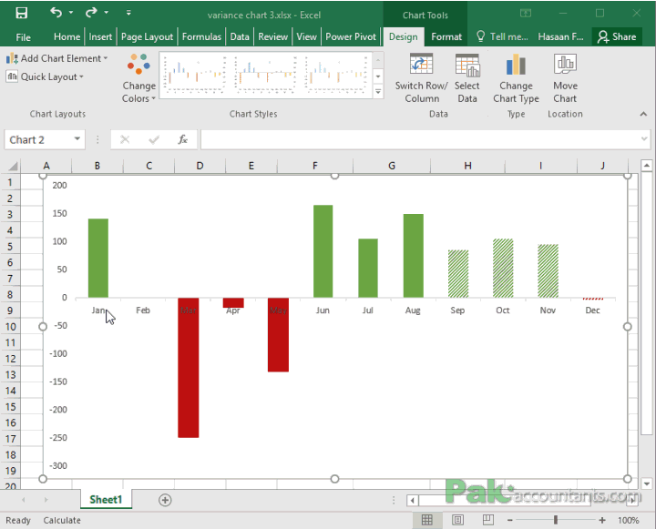
Excel bar chart with conditional formatting based on MoM ... Conditional formatting of Excel charts allows you to have the formatting of the chart update automatically based on the data values.

Excel Course: Inserting Graphs

Conditional formatting chart data labels? - Excel Help Forum The easy way to conditionally format these labels is use two series. Use something like =IF ($E2=1,0,NA ()) for the series that has red labels and =IF (#E2=1,NA (),0) for the series that has unformatted labels. Jon Peltier Register To Reply Similar Threads Conditional Number Formatting Not Working for Chart Value Labels

Share :