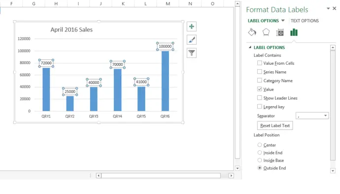
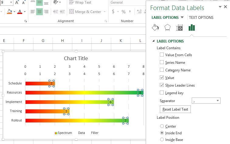
40 move data labels excel chart
Topics with Label: Connecting to Data - Power Platform Community Join the discussion. Showing topics with label Connecting to Data. Show all topics. Descriptive data analysis: COUNT, SUM, AVERAGE, and other calculations STEPS: 1. In your "Calculations" worksheet, select the entire table with the data you have calculated for sex. Copy this table (either click the "copy" button in the top left hand corner of your "Home" menu, or right-click where you have selected the table and click "copy"). 2.
Excel Tips & Solutions Since 1998 - MrExcel Publishing Strategy: There is an alternate way to specify the third argument. Instead of specifying 1-7 or 11-17, you can specify a 7-digit text string comprised of 1's and 0's. The first character in the text is Monday. The seventh character is Sunday. Remember the name of this argument is [weekend].
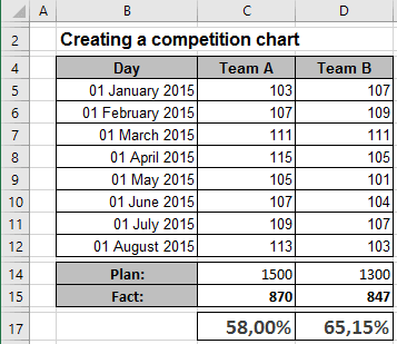
Move data labels excel chart
Excel Pivot Table Index for Contextures Website Tutorials Interactive Excel Pivot Table Demo. Adjust the Field List. Pivot FAQs. Pivot Table Select ... Move Row Labels in Pivot Table. Pivot Items. Remove Old Items. Show/Hide Items. Value Fields. Data Fields ... Pivot Chart Macros. Source Data and Refresh. Automatically Include New Data. DrillDown (Show Details) ... improve your graphs, charts and data visualizations — storytelling with ... To adjust the x-axis to show the years, right-click on the chart and go to Select Data… in the pop-up menu. Campaign Year and Meals Served are in the list in the series box in the middle. Pick Campaign Year and then click the minus (-) sign box below the list to remove Campaign Year as a series. Displaying Long Text Fields in Tableau from Excel - InterWorks Third Part: =MID (C2, 512, 255) Ex. 3 - The resulting columns parse the original Long Description field and only keep the parts limited by the formulas. After saving the spreadsheet, refresh the view in Tableau. In order to get all of the parts of the Long Description into one field, common sense would say to simple concatenate the three ...
Move data labels excel chart. Use ribbon charts in Power BI - Power BI | Microsoft Docs By default, borders are off. Since the ribbon chart does not have y-axis labels, you may want to add data labels. From the Formatting pane, select Data labels. Set formatting options for your data labels. In this example, we've set the text color to white and display units to thousands. Next steps Scatter charts and bubble charts in Power BI Tableau Essentials: Chart Types - Packed Bubbles - InterWorks Let's expand our data set to see more bubbles on the screen in a single view so we can get a better idea of how a packed bubble chart organizes a larger scope of data. Above, I added State to Detail to add more information to the first bubble chart. Now, we get one bubble per Product , Product Type and State. Note the arrangement of the bubbles. 8 Excel Pivot Table Examples - How to Make PivotTables - ExcelDemy When Amount data is placed in the Rows section, data is placed ungrouped. To make data in the group, click the Group option as per this image. Select Group from the options, the Grouping dialog box will appear. Enter 1, 100000, and 5000 in three fields respectively. Grouping data with the help of the Grouping dialog box. Best Online Excel Classes of 2022 - Investopedia For those who prefer to learn on the move, GoSkills' classes are ideal. Microsoft Excel Classes—Basic and Advanced makes our list because it's available on IOS and Android devices. It ...
How to Create Excel Pivot Table (Includes practice file) Mixed data formats will pose a problem. Click any populated cell. This helps set the range. Highlight your data range. Tip: You can press Ctrl + A to select all. Click the Insert tab. Your toolbar groups will change. Select the PivotTable button from the Tables group. This should be the first group. The Create PivotTable dialog appears. My Charts - Barchart.com The "My Charts" feature, available to Barchart Premier Members, lets you build a portfolio of personalized charts that you can view on demand. Save numerous chart configurations for the same symbol, each with their own trendlines and studies. Save multiple commodity spread charts and expressions, view quote and technical analysis data, and more ... Blank Labels on Sheets for Inkjet/Laser - OnlineLabels Item: OL6950BK - 2.25" x 0.75" Labels | Brown Kraft (Laser and Inkjet) By Jenna on June 1, 2022. We use several different sizes depending on what we're labeling. The quality is great, the ordering process is a breeze, the delivery is ridiculously fast, and the price is right!!! Can't go wrong! Radial gauge charts in Power BI - Power BI | Microsoft Docs Select financials and Sheet1 Click Load Select to add a new page. Create a basic radial gauge Step 1: Create a gauge to track Gross Sales Start on a blank report page From the Fields pane, select Gross Sales. Change the aggregation to Average. Select the gauge icon to convert the column chart to a gauge chart.
PowerChurch - Church Management Software for Today's Growing Churches Church Management Software has never been so affordable or easy to use! PowerChurch Plus makes it easy to manage your membership, non-profit accounting, and contribution information. Customize X-axis and Y-axis properties - Power BI You can add and modify the data labels, Y-axis title, and gridlines. For values, you can modify the display units, decimal places, starting point, and end point. And, for categories, you can modify the width, size, and padding of bars, columns, lines, and areas. The following example continues our customization of a column chart. 1.131 FAQ-719 How to adjust line space betwen lines in the Legend? - Origin Last Update: 10/16/2016. If you want to adjust the line space between lines in the legend, you can right-click the legend to select Properties... from the context menu to open the Text Object dialog. In the Text tab of this dialog, for the Line Spacing (%) item, select a value from the drop-down list or enter a value in the combo box directly. 3 Ways to Convert Scanned PDF to Excel - Wondershare PDFelement PDFelement enables you to convert multiple scanned PDFs to excel in a batch, which can help you save time and effort a lot. Try It Free Step 1. After opening PDFelement, click the "Batch Process" button to get access. Step 2. In the "Convert" tab, you can add multiple scanned PDF files to it. And choose Excel in the "Output Format" option.
Creating a chart with dynamic labels - Microsoft Excel 2016
The 8 Best Label Makers of 2022 - The Spruce Measuring 8 x 4 x 2 inches and weighing only 1.4 pounds, the LabelManager 280 is conveniently compact and portable as well, but also an excellent choice for at-home use. It runs on a rechargeable battery and is able to print labels that are 0.25, 0.375, or 0.5 inches wide.
Excel Chart: Dynamic Data Label - YouTube
Get started formatting Power BI visualizations - Power BI With the same clustered column chart selected, expand the Effects > Background options. Move the Background slider to On. Select the drop-down and choose a grey color. Change Transparency to 74%. At this point in the tutorial, your clustered column chart background will look something like this:
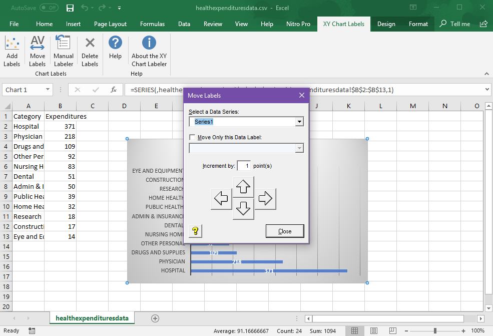
Add Labels to XY Chart Data Points in Excel with XY Chart Labeler
Data networks and IP addresses: View as single page - Open University A computing device will evaluate the IP address and subnet mask together, bit by bit (this is called bit wise), performing a logical 'AND' operation: Figure 5. The AND function will take two inputs, and if they are both '1', it will output a '1'. Any other combination of inputs will result in a '0' output.

How to Create a Chart in Microsoft Excel - Tech Support
Treemaps in Power BI - Power BI | Microsoft Docs From the Fields pane, select the Sales > Last Year Sales measure. Select the treemap icon to convert the chart to a treemap. Select Item > Category which will add Category to the Group well. Power BI creates a treemap where the size of the rectangles is based on total sales and the color represents the category.

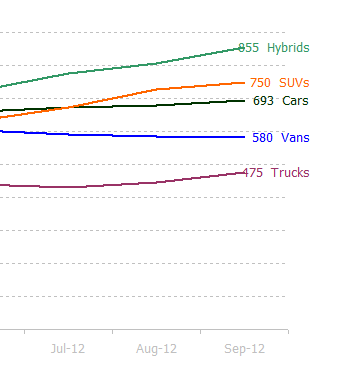
Directly Labeling Excel Charts | PolicyViz
How to add secondary axis in Excel (2 easy ways) - ExcelDemy Let's change the chart type. Go to Design tab (shows only when the chart is selected) => Type window => and click on the Change Chart Type command 5) Change Chart Type dialog box appears. This dialog box is actually our old Insert Chart dialog box. The Combo option is already selected.
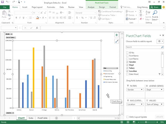
How to Create Pivot Charts in Excel 2016 - dummies
Leader Lines in Excel Pie Charts - Microsoft Community I've created pie charts in Excel. When I move the labels around I get leader lines that I do not want. I can delete them but if I save, close and then open the file, they come back. I can format the lines so that the color is white and they do not show. But again, if I save, close and reopen, the lines turn back to black.

Chart Data Labels in PowerPoint 2011 for Mac
5 Tableau Table Calculation Functions That You Need to Know This function returns a 0 for the first visible row and then negative incremental numbers for the following rows or partitions. LAST () This function, obviously the opposite of FIRST (), returns a 0 for the last visible row and then positive incremental numbers for the subsequent rows.
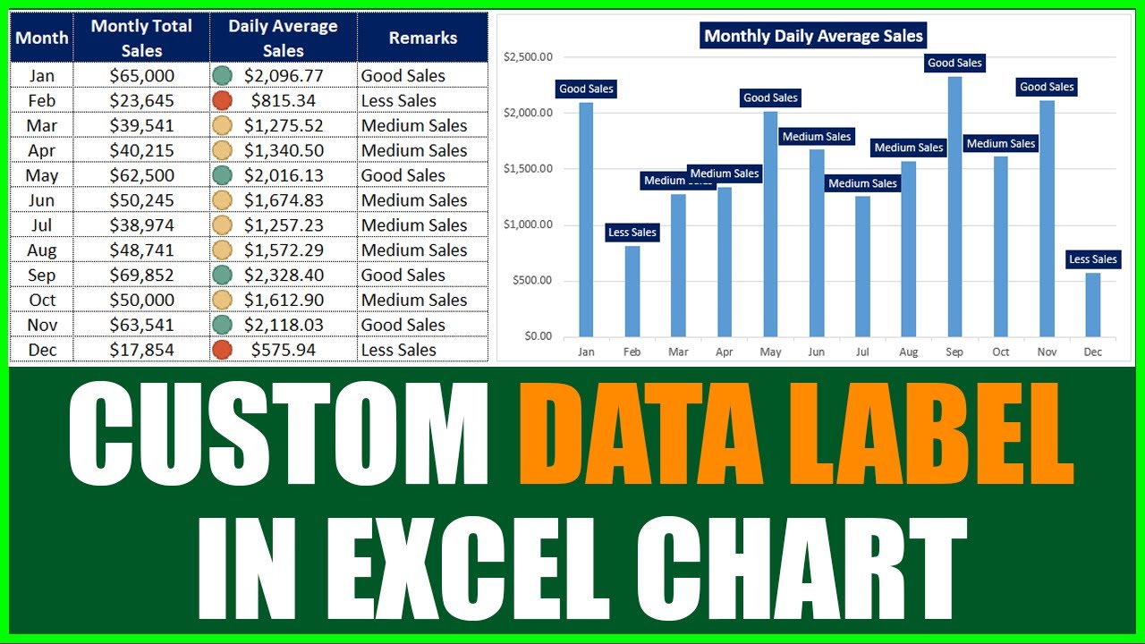
Formula Friday - Using Formulas To Add Custom Data Labels To Your Excel Chart - How To Excel At ...
A Solution to Tableau Line Charts with Missing Data Points We need to click on the Date pill and select Show Missing Values: With our new calculated field, we see a nice continuous line as opposed to the stop/start view of the original field: So, there we have it - a nice, quick and easy way to fill your data out and get a fuller picture of line charts.
Excel Dashboard Templates New Take on the Excel Project Status Spectrum Chart - Excel Dashboard ...
Using MarcEdit to Convert .mrc File to Tab Delimited File for Excel ... Data Processing Toggle Dropdown. Create a spreadsheet from Print 03 ; ... E-Z* moving of order and holdings records ; Serials Toggle Dropdown. Abbreviations for Captions ; ... Using MarcEdit to Convert .mrc File to Tab Delimited File for Excel. Once the MARC files have been retrieved, they can be converted into a tab delimited file that can be ...

How to make a pie chart in Excel
what is a stacked bar chart? — storytelling with data Move data labels inside the ends of bars. Don't truncate the length of the bars. You can read more of these fundamental tips in the what is a bar chart guide. Here are a few more stacked-bar-specific considerations to be mindful of as well. Place the most important stack along the baseline

How to Add Data Labels to your Excel Chart in Excel 2013 - YouTube
Displaying Long Text Fields in Tableau from Excel - InterWorks Third Part: =MID (C2, 512, 255) Ex. 3 - The resulting columns parse the original Long Description field and only keep the parts limited by the formulas. After saving the spreadsheet, refresh the view in Tableau. In order to get all of the parts of the Long Description into one field, common sense would say to simple concatenate the three ...

Surface Chart in Excel
improve your graphs, charts and data visualizations — storytelling with ... To adjust the x-axis to show the years, right-click on the chart and go to Select Data… in the pop-up menu. Campaign Year and Meals Served are in the list in the series box in the middle. Pick Campaign Year and then click the minus (-) sign box below the list to remove Campaign Year as a series.
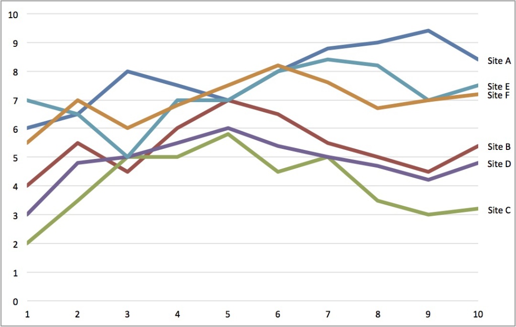
Directly Labeling Excel Charts - PolicyViz
Excel Pivot Table Index for Contextures Website Tutorials Interactive Excel Pivot Table Demo. Adjust the Field List. Pivot FAQs. Pivot Table Select ... Move Row Labels in Pivot Table. Pivot Items. Remove Old Items. Show/Hide Items. Value Fields. Data Fields ... Pivot Chart Macros. Source Data and Refresh. Automatically Include New Data. DrillDown (Show Details) ...
Placing Chart Data Labels – Daily Dose of Excel

Create a Clustered AND Stacked column chart in Excel (easy)
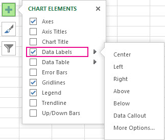
Move data labels - Office Support

After formatting each label, you can delete the legend and style the gridlines, tick marks, etc ...
Post a Comment for "40 move data labels excel chart"