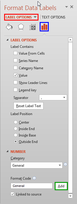
38 format data labels pane excel
Add a DATA LABEL to ONE POINT on a chart in Excel You can now configure the label as required — select the content of the label (e.g. series name, category name, value, leader line), the position (right, left, above, below) in the Format Data Label pane/dialog box. To format the font, color and size of the label, now right-click on the label and select 'Font'. Note: in step 5. above, if ... Excel 2016 Tutorial Formatting Data Labels Microsoft Training Lesson FREE Course! Click: about Formatting Data Labels in Microsoft Excel at . A clip from Mastering Excel M...
Format Data Labels in Excel- Instructions - TeachUcomp, Inc. To do this, click the "Format" tab within the "Chart Tools" contextual tab in the Ribbon. Then select the data labels to format from the "Chart Elements" drop-down in the "Current Selection" button group. Then click the "Format Selection" button that appears below the drop-down menu in the same area.
Format data labels pane excel
Formatting data labels and printing pie charts on Excel for Mac 2019 ... Here's a work around I found for printing pie charts. Still can't find a solution for formatting the data labels. 1. When printing a pie chart from Excel for mac 2019, MS instructions are to select the chart only, on the worksheet > file > print. Excel is supposed to print the chart only (not the data ) and automatically fit it onto one page. Excel 2019 & 365 Tutorial Formatting Data Labels Microsoft Training FREE Course! Click: Learn about Formatting Data Labels in Microsoft Excel at . A clip from Mastering Excel ... How to hide zero data labels in chart in Excel? In the Format Data Labelsdialog, Click Numberin left pane, then selectCustom from the Categorylist box, and type #""into the Format Codetext box, and click Addbutton to add it to Typelist box. See screenshot: 3. Click Closebutton to close the dialog. Then you can see all zero data labels are hidden.
Format data labels pane excel. How to Create Mailing Labels in Excel | Excelchat B. If we do this, when next we open the document, MS Word will ask where we want to merge from Excel data file. We will click Yes to merge labels from Excel to Word. Figure 26 - Print labels from excel (If we click No, Word will break the connection between document and Excel data file.) C. Alternatively, we can save merged labels as usual text. HOW TO STAGGER AXIS LABELS IN EXCEL - simplexCT 21. In the chart, right click the Horizontal (Category) Axis and on the shortcut menu click Format Axis. 22. In the Format Axis pane, under Labels, set the Labels Position to None. 23. Click the Fill & Line icon and select Solid Line under Line and set the Color to Black and the Width to 1.5. 24. Excel Charts - Aesthetic Data Labels - tutorialspoint.com To format the data labels − Step 1 − Right-click a data label and then click Format Data Label. The Format Pane - Format Data Label appears. Step 2 − Click the Fill & Line icon. The options for Fill and Line appear below it. Step 3 − Under FILL, Click Solid Fill and choose the color. Excel tutorial: The Format Task pane You can also select a chart element first, then use the keyboard shortcut Control + 1. For example, if I select the data bars in this chart, then type Control + 1, the Format Task Pane will open with with the data series options selected. The Format Task pane stays open until you manually close the window.
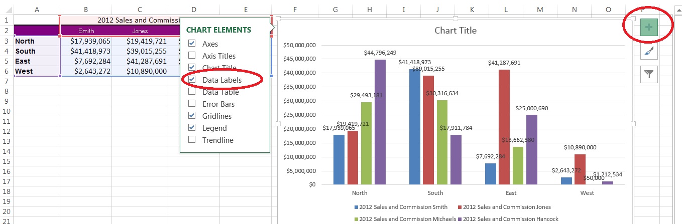
How to Customize Your Excel Pivot Chart Data Labels - dummies Excel displays the Format Data Labels pane. Check the box that corresponds to the bit of pivot table or Excel table information that you want to use as the label. For example, if you want to label data markers with a pivot table chart using data series names, select the Series Name check box. How to Add Data Labels to an Excel 2010 Chart - dummies Excel provides several options for the placement and formatting of data labels. Use the following steps to add data labels to series in a chart: Click anywhere on the chart that you want to modify. On the Chart Tools Layout tab, click the Data Labels button in the Labels group. A menu of data label placement options appears: None: The default ... Excel Charts - Quick Formatting - tutorialspoint.com The Format pane by default appears on the right-side of the chart. Step 1 − Click on the chart. Step 2 − Right-click the horizontal axis. A drop-down list appears. Step 3 − Click Format Axis. The Format pane for formatting axis appears. The format pane contains the task pane options. Step 4 − Click the Task Pane Options icon. Format Data Label: Label Position - Microsoft Community when you add labels with the + button next to the chart, you can set the label position. In a stacked column chart the options look like this: For a clustered column chart, there is an additional option for "Outside End" When you select the labels and open the formatting pane, the label position is in the series format section. Does that help?
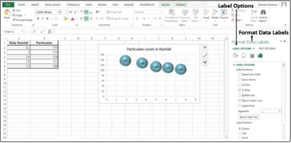
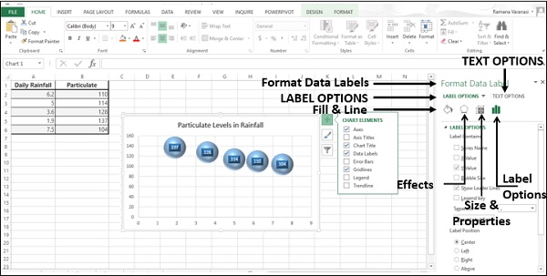
Excel tutorial: How to use data labels When first enabled, data labels will show only values, but the Label Options area in the format task pane offers many other settings. You can set data labels to show the category name, the series name, and even values from cells. In this case for example, I can display comments from column E using the "value from cells" option. How to add data labels from different column in an Excel chart? Right click the data series, and select Format Data Labels from the context menu. 3. In the Format Data Labels pane, under Label Options tab, check the Value From Cells option, select the specified column in the popping out dialog, and click the OK button. Now the cell values are added before original data labels in bulk. 4. Change the format of data labels in a chart To get there, after adding your data labels, select the data label to format, and then click Chart Elements > Data Labels > More Options. To go to the appropriate area, click one of the four icons ( Fill & Line, Effects, Size & Properties ( Layout & Properties in Outlook or Word), or Label Options) shown here. Pie Chart in Excel - Inserting, Formatting, Filters, Data Labels Right click on the Data Labels on the chart. Click on Format Data Labels option. Consequently, this will open up the Format Data Labels pane on the right of the excel worksheet. Mark the Category Name, Percentage and Legend Key. Also mark the labels position at Outside End. This is how the chark looks. Formatting the Chart Background, Chart Styles
Label Options for Chart Data Labels in PowerPoint 2013 for Windows
How do you format data series in Excel? To format data labels in EÎl , choose the set of data labels to format . To do this, click the " Format " tab within the "Chart Tools" contextual tab in the Ribbon. Then select the data labels to format from the "Chart Elements" drop-down in the "Current Selection" button group. How do I show the Format Data Series pane in Excel?
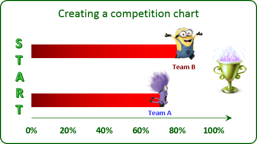
Creating a simple competition chart - Microsoft Excel 2013
How to Print Labels from Excel - Lifewire Select Mailings > Write & Insert Fields > Update Labels . Once you have the Excel spreadsheet and the Word document set up, you can merge the information and print your labels. Click Finish & Merge in the Finish group on the Mailings tab. Click Edit Individual Documents to preview how your printed labels will appear. Select All > OK .
Quick Tip: Excel 2013 offers flexible data labels - TechRepublic
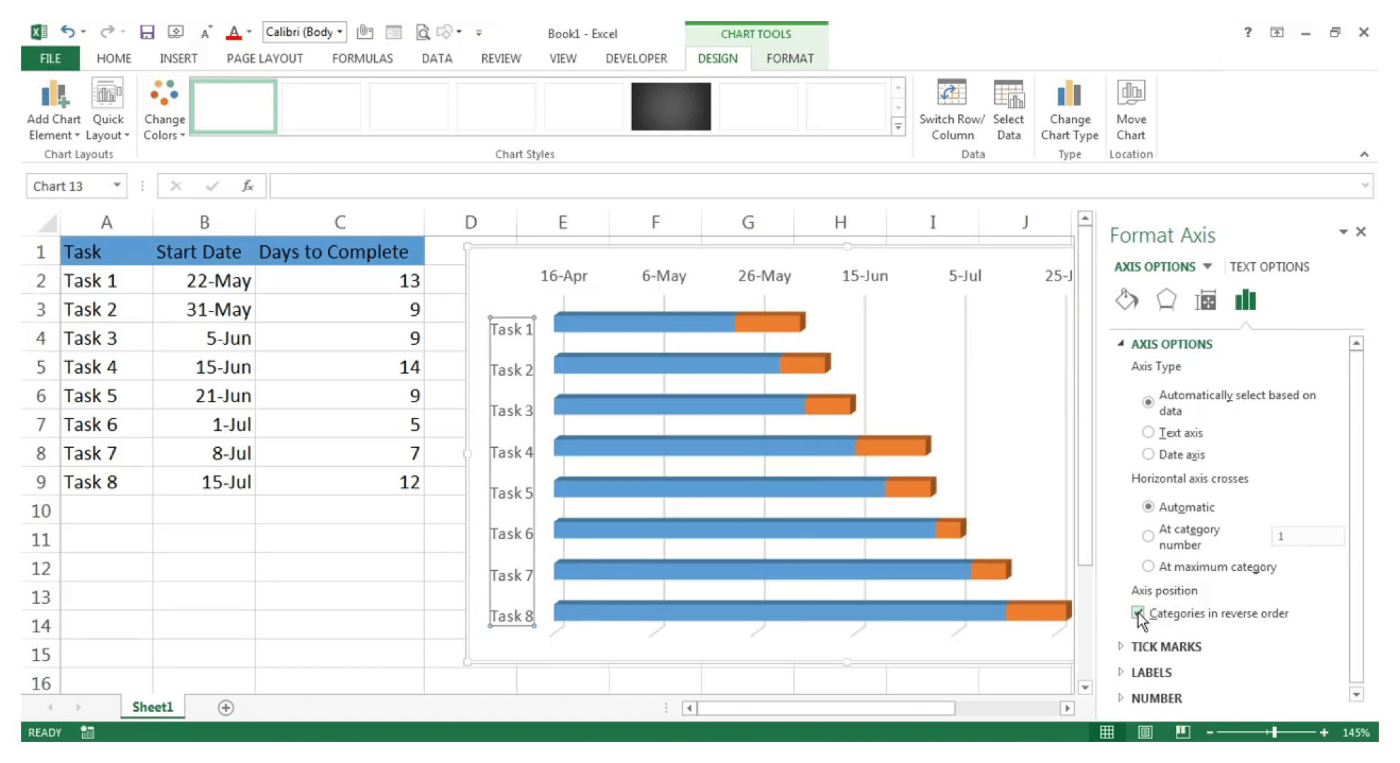
Format Chart Axis in Excel - Axis Options Analyzing Format Axis Pane. Right-click on the Vertical Axis of this chart and select the "Format Axis" option from the shortcut menu. This will open up the format axis pane at the right of your excel interface. Thereafter, Axis options and Text options are the two sub panes of the format axis pane.

Format Data Label Options for Charts in PowerPoint 2011 for Mac
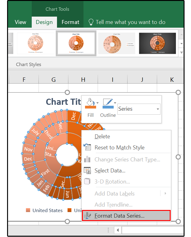
Using Graphics to Represent Data Series (Microsoft Excel) Choose Format Data Series from the Context menu. Excel displays the Format Data Series task pane at the right side of the chart. In the task pane click the Fill & Line icon; it looks like a spilling paint bucket. Expand the Fill options by clicking the small triangle next to the Fill heading. (See Figure 2.) Figure 2. The Fill options of the ...
GNIIT HELP: Advanced Excel - Richer Data Labels ~ GNIITHELP
Format elements of a chart - support.microsoft.com Right-click the chart axis, and click Format Axis. In the Format Axis task pane, make the changes you want. You can move or resize the task pane to make working with it easier. Click the chevron in the upper right. Select Move and then drag the pane to a new location. Select Size and drag the edge of the pane to resize it.

Advanced Excel Richer Data Labels in Advanced Excel Functions Tutorial 03 December 2020 - Learn ...
How to Print Labels From Excel - EDUCBA Navigate towards the folder where the excel file is stored in the Select Data Source pop-up window. Select the file in which the labels are stored and click Open. A new pop up box named Confirm Data Source will appear. Click on OK to let the system know that you want to use the data source. Again a pop-up window named Select Table will appear.

Format Data Labels in Excel- Instructions - TeachUcomp, Inc.
How to hide zero data labels in chart in Excel? In the Format Data Labelsdialog, Click Numberin left pane, then selectCustom from the Categorylist box, and type #""into the Format Codetext box, and click Addbutton to add it to Typelist box. See screenshot: 3. Click Closebutton to close the dialog. Then you can see all zero data labels are hidden.

Format Data Label Options for Charts in PowerPoint 2013 for Windows
Excel 2019 & 365 Tutorial Formatting Data Labels Microsoft Training FREE Course! Click: Learn about Formatting Data Labels in Microsoft Excel at . A clip from Mastering Excel ...

How to make a histogram in Excel 2019, 2016, 2013 and 2010
Formatting data labels and printing pie charts on Excel for Mac 2019 ... Here's a work around I found for printing pie charts. Still can't find a solution for formatting the data labels. 1. When printing a pie chart from Excel for mac 2019, MS instructions are to select the chart only, on the worksheet > file > print. Excel is supposed to print the chart only (not the data ) and automatically fit it onto one page.

Format Data Labels in Excel 2013- Tutorial - TeachUcomp, Inc.
Excel 2016 charts: How to use the new Pareto, Histogram, and Waterfall formats | PCWorld
Excel Dashboards - Краткое руководство - CoderLessons.com

How to create an Excel map chart

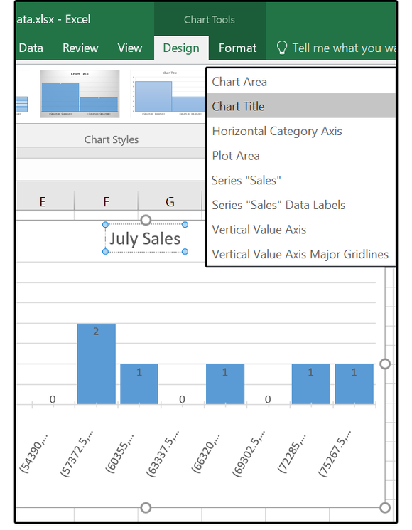
Excel Chart Elements: Parts of Charts in Excel | ExcelDemy
How to Make Gantt Chart in Excel? | Gantt Chart Excel - Zoho Projects
What to do with Excel 2016's new chart styles: Treemap, Sunburst, and Box & Whisker | PCWorld

format-data-labels | Real Statistics Using Excel
Post a Comment for "38 format data labels pane excel"