44 add data labels to pivot chart

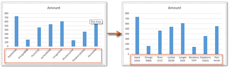
How to Add Filter to Pivot Table: 7 Steps (with Pictures) - wikiHow Mar 28, 2019 · Pivot tables can provide a great deal of information and analysis about the data contained in a worksheet, but, sometimes, even the most well-designed pivot table can display more information than you need. In these cases, it can be helpful to set up filters within your pivot table. Filters can be set up once and then changed as needed to display different information … › office-addins-blog › 2015/10/29Excel charts: add title, customize chart axis, legend and ... Oct 29, 2015 · Click the Chart Elements button, and select the Data Labels option. For example, this is how we can add labels to one of the data series in our Excel chart: For specific chart types, such as pie chart, you can also choose the labels location. For this, click the arrow next to Data Labels, and choose the option you want.

How to add Data label in Stacked column chart of Pivot charts I'm tring to make a Pivot chart with stacked column graph. In where, i couldn't add data label for cumulative sum of value in Data label. Where i could only add data label to individual stacks in column graph. It found possible with normal stacked column chart without pivot chart.

Add data labels to pivot chart

support.google.com › docs › answerAdd & edit a chart or graph - Computer - Google Docs Editors Help Double-click the chart you want to change. At the right, click Customize. Click Gridlines. Optional: If your chart has horizontal and vertical gridlines, next to "Apply to," choose the gridlines you want to change. Make changes to the gridlines. Tips: To hide gridlines but keep axis labels, use the same color for the gridlines and chart background. How to Add Two Data Labels in Excel Chart (with Easy Steps) Step 4: Format Data Labels to Show Two Data Labels. Here, I will discuss a remarkable feature of Excel charts. You can easily show two parameters in the data label. For instance, you can show the number of units as well as categories in the data label. To do so, Select the data labels. Then right-click your mouse to bring the menu. Add & edit a chart or graph - Computer - Google Docs Editors … Double-click the chart you want to change. At the right, click Customize. Click Gridlines. Optional: If your chart has horizontal and vertical gridlines, next to "Apply to," choose the gridlines you want to change. Make changes to the gridlines. Tips: To hide gridlines but keep axis labels, use the same color for the gridlines and chart background.

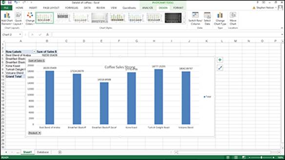
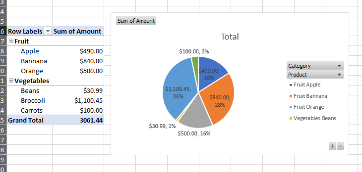
Add data labels to pivot chart. Data Labels in Excel Pivot Chart (Detailed Analysis) Before adding the Data Labels, we need to create the Pivot Chart in the beginning. We can create a Pivot Chart from the Insert tab. To do this, go to Insert tab > Tables group. Then in the dialog box, select the range of cells of the primary dataset., here the range of cells is B4:J23. And select the New Worksheet in the next option. › Add-Filter-to-Pivot-TableHow to Add Filter to Pivot Table: 7 Steps (with Pictures) Mar 28, 2019 · The attribute should be one of the column labels from the source data that is populating your pivot table. For example, assume your source data contains sales by product, month and region. You could choose any one of these attributes for your filter and have your pivot table display data for only certain products, certain months or certain regions. How To Add Another Row Labels In Pivot Table - Brokeasshome.com Breaking News. How To Add Another Row Labels In Pivot Table; How To Add One More Row In Pivot Table; How To Add A Calculated Column In Pivot Table Excel 2017 How do I add labels to my pivot chart? - Firstlawcomic Select the plot area of the pie chart. Right-click the chart. Select Add Data Labels. Select Add Data Labels. In this example, the sales for each cookie is added to the slices of the pie chart. How do you change the axis labels on a pivot chart? Right-click the category labels you want to change, and click Select Data. In the Horizontal ...

Pivot Chart Formatting Changes When Filtered - Peltier Tech Apr 07, 2014 · I have a pivot chart based on data collected from a customer survey for 5 different customer bases (EUROPE, SOUTH AMERICA, ASIA, etc). ... You have to remove labels completely and add them once again. Seems it’s not pivot itself causing problems but chart freaks out when ranges are changing. Jon Peltier says. Friday, December 9, 2016 at 11:53 am. Research Service - LRS.org Jul 28, 2022 · Hello data enthusiasts! Let’s return to our exploration of qualitative analysis. Last time we uncovered a few ways qualitative analysis can expand research findings by looking beyond number data for better insight on human experiences. Now I want to explore strategies for putting qualitative analysis into practice. Add data and format Pivot Chart using VBA Excel I tried the recorder after my initial attempts failed. I have also failed to have the ChartTitle.Add work so I can amend the title that is visible (Currently nothing shows as a title). ActionTracker.PivotCaches.Create (SourceType:=xlDatabase, SourceData:= _ Actions, Version:=6).CreatePivotTable _ TableDestination:=CtyDrng, TableName:="Country ... Add a DATA LABEL to ONE POINT on a chart in Excel Steps shown in the video above: Click on the chart line to add the data point to. All the data points will be highlighted. Click again on the single point that you want to add a data label to. Right-click and select ' Add data label ' This is the key step! Right-click again on the data point itself (not the label) and select ' Format data label '.

Library Research Service - LRS.org Jul 28, 2022 · Hello data enthusiasts! Let’s return to our exploration of qualitative analysis. Last time we uncovered a few ways qualitative analysis can expand research findings by looking beyond number data for better insight on human experiences. Now I want to explore strategies for putting qualitative analysis into practice. Add a data label on Pivot Chart - social.technet.microsoft.com With ActiveChart With .SeriesCollection (1).Points (i) .HasDataLabel = True .DataLabel.Text = Worksheets ("Sheet2").Range ("a" & position_total).Value position_total = position_total + 1 End With End With Next End Sub Select the Pivot chart, then run the macro "data_label". Jaynet Zhang TechNet Community Support Monday, April 30, 2012 4:50 AM › charts › dynamic-chart-dataCreate Dynamic Chart Data Labels with Slicers - Excel Campus You basically need to select a label series, then press the Value from Cells button in the Format Data Labels menu. Then select the range that contains the metrics for that series. Click to Enlarge Repeat this step for each series in the chart. If you are using Excel 2010 or earlier the chart will look like the following when you open the file. Pivot Chart Data Label Help Needed - Microsoft Community Open the Excel file with Pivot Chart and enabled with Data Labels> Click on the Labels displayed in the Chart> Right-click> Click Format Data Labels> Label Options> Number> In the Category, select the format as per your requirement. Here is the reference article: Change the format of data labels in a chart.

Creating Databound ADF Data Visualization Components

How to add data labels from different column in an Excel chart? Right click the data series in the chart, and select Add Data Labels > Add Data Labels from the context menu to add data labels. 2. Click any data label to select all data labels, and then click the specified data label to select it only in the chart. 3.

How to Create Progress Charts (Bar and Circle) in Excel - Automate Excel

Add or remove data labels in a chart - support.microsoft.com To label one data point, after clicking the series, click that data point. In the upper right corner, next to the chart, click Add Chart Element > Data Labels. To change the location, click the arrow, and choose an option. If you want to show your data label inside a text bubble shape, click Data Callout.

Use Google Forms to Make a Pivot Chart - TechnoKids Blog

Add Value Label to Pivot Chart Displayed as Percentage If you use the hidden line method: How to Add Total Data Labels to the Excel Stacked Bar Chart and then use the code mentioned in post #2 to create boxes offset from the hidden line points, you should be able to place the additional labels where you want. You must log in or register to reply here. Similar threads E

How to wrap X axis labels in a chart in Excel?

chandoo.org › wp › change-data-labels-in-chartsHow to Change Excel Chart Data Labels to Custom Values? May 05, 2010 · First add data labels to the chart (Layout Ribbon > Data Labels) Define the new data label values in a bunch of cells, like this: Now, click on any data label. This will select “all” data labels. Now click once again. At this point excel will select only one data label.

How to group (two-level) axis labels in a chart in Excel?

How to add data labels to pivot chart? - Syncfusion The CSV data goes into the Data sheet and the application then creates a pivot table and corresponding pivot chart from this data in the Charts sheet. The chart is created alright but i see no option to add data labels to it using XlsIO. The chart is created as follows: IChartShape pivotChart = chartsSheet.Charts.Add();

image

Origin: Data Analysis and Graphing Software An add labels option is also available to facilitate adding labels to each unit in the merged graph. Options in Plot Details Layer tab enable users to automatically ... In this grouped box chart, labels representing the group variables have been created ... and pivot tables; Data protection by disable editing; Save import settings, format and ...

MS Excel 2013: Display the fields in the Values Section in multiple columns in a pivot table

How to Customize Your Excel Pivot Chart Data Labels - dummies To add data labels, just select the command that corresponds to the location you want. To remove the labels, select the None command. If you want to specify what Excel should use for the data label, choose the More Data Labels Options command from the Data Labels menu. Excel displays the Format Data Labels pane.

How-to Use Data Labels from a Range in an Excel Chart - Excel Dashboard Templates

peltiertech.com › copy-pivot-table-pivot-chartCopy a Pivot Table and Pivot Chart and Link to New Data Jul 15, 2010 · Hello, I was trying to follow the steps listed in the “Copy a Pivot Table and Pivot Chart and Link to New Data” article, but after re-linking the copied pivotchart, excel 2007 simply remove the old pivotchart formating (colors, labels, captions, etc).

Problems formatting pivot chart data labels in Mac v16 - Microsoft Tech Community

Excel Power Pivot - Loading Data - tutorialspoint.com In this chapter, we will learn to load data into Power Pivot. You can load data into Power Pivot in two ways −. Load data into Excel and add it to the Data Model. Load data into PowerPivot directly, populating the Data Model, which is the PowerPivot database. If you want the data for Power Pivot, do it the second way, without Excel even ...

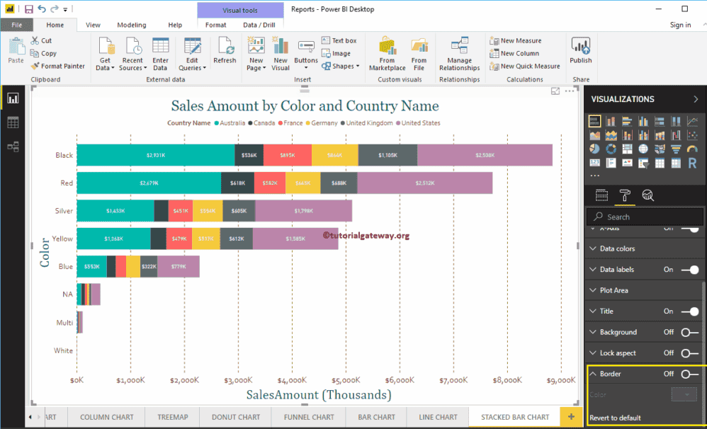
Format Stacked Bar Chart in Power BI

EOF

Add label to Excel chart line • AuditExcel.co.za

Copy a Pivot Table and Pivot Chart and Link to New Data Jul 15, 2010 · This action, of moving the chart or pivot table will add an absolute path to the data source : ‘Book1 only pivot table.xlsx’!Table1. ... behaviors are different than if you simply use worksheet data. In any case, if you modify the header labels in pivot source data, you risk breaking the structure of the pivot table and chart.

Pivot Chart Data Label Help Needed - Microsoft Community

Adding Data Labels to a Chart Using VBA Loops - Wise Owl To do this, add the following line to your code: 'make sure data labels are turned on. FilmDataSeries.HasDataLabels = True. This simple bit of code uses the variable we set earlier to turn on the data labels for the chart. Without this line, when we try to set the text of the first data label our code would fall over.

Working with Multiple Data Series in Excel | Pryor Learning Solutions

How to Add Data to a Pivot Table: 11 Steps (with Pictures) - wikiHow You can do this in both Windows and Mac versions of Excel. Steps Download Article 1 Open your pivot table Excel document. Double-click the Excel document that contains your pivot table. It will open. 2 Go to the spreadsheet page that contains your data. Click the tab that contains your data (e.g., Sheet 2) at the bottom of the Excel window. 3

How To Use Dynamic Data Labels To Create Interactive Excel Charts

Create Dynamic Chart Data Labels with Slicers - Excel Campus Feb 10, 2016 · This includes using the XY Chart Labeler Add-in, which is a free download for Windows or Mac. Step 6: Setup the Pivot Table and Slicer. The final step is to make the data labels interactive. We do this with a pivot table and slicer. The source data for the pivot table is the Table on the left side in the image below.

How to Add Total Data Labels to the Excel Stacked Bar Chart – MBA Excel

How to change/edit Pivot Chart's data source/axis ... - ExtendOffice Step 1: Select the Pivot Chart you will change its data source, and cut it with pressing the Ctrl + X keys simultaneously. Step 2: Create a new workbook with pressing the Ctrl + N keys at the same time, and then paste the cut Pivot Chart into this new workbook with pressing Ctrl + V keys at the same time. Step 3: Now cut the Pivot Chart from ...

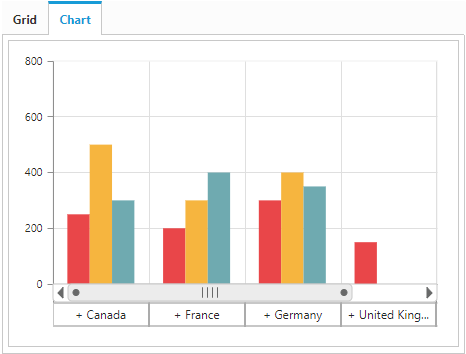
Pivot Chart | ASP.NET Web Forms Pivot and OLAP browser | Syncfusion

Excel charts: add title, customize chart axis, legend and data labels Oct 29, 2015 · Click the Chart Elements button, and select the Data Labels option. For example, this is how we can add labels to one of the data series in our Excel chart: For specific chart types, such as pie chart, you can also choose the labels location. For this, click the arrow next to Data Labels, and choose the option you want.

Share :