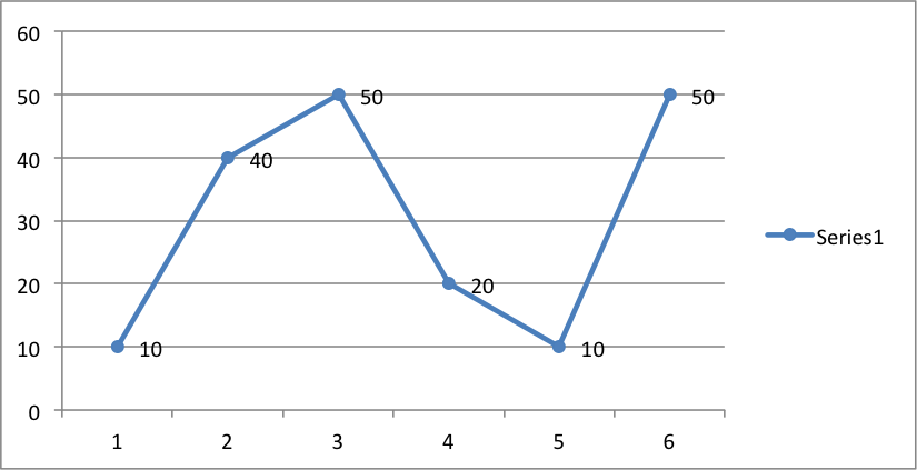
39 excel graph data labels different series

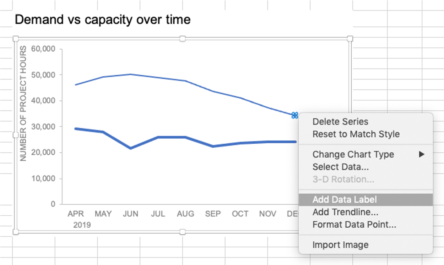
how to add data labels into Excel graphs - storytelling with data You can download the corresponding Excel file to follow along with these steps: Right-click on a point and choose Add Data Label. You can choose any point to add a label—I'm strategically choosing the endpoint because that's where a label would best align with my design. Excel defaults to labeling the numeric value, as shown below. Add a DATA LABEL to ONE POINT on a chart in Excel All the data points will be highlighted. Click again on the single point that you want to add a data label to. Right-click and select ' Add data label '. This is the key step! Right-click again on the data point itself (not the label) and select ' Format data label '. You can now configure the label as required — select the content of ...

Label line chart series - Get Digital Help To label each line we need a cell range with the same size as the chart source data. Simply copy the chart source data range and paste it to your worksheet, then delete all data. All cells are now empty. Copy categories (Regions in this example) and paste to the last column (2018). Those correspond to the last data points in each series.

Excel graph data labels different series

How to Use Cell Values for Excel Chart Labels - How-To Geek Select the chart, choose the "Chart Elements" option, click the "Data Labels" arrow, and then "More Options." Uncheck the "Value" box and check the "Value From Cells" box. Select cells C2:C6 to use for the data label range and then click the "OK" button. The values from these cells are now used for the chart data labels. Change the format of data labels in a chart You can add a built-in chart field, such as the series or category name, to the data label. But much more powerful is adding a cell reference with explanatory text or a calculated value. Click the data label, right click it, and then click Insert Data Label Field. If you have selected the entire data series, you won't see this command. Formating all data labels in a single series at once. Easiest way to make sure you are doing the right thing is to click off the data labels but on the chart and then right click any data label and choose Format Data Labels. Note the choice on the shortcut menu should not say Format Data Label. What's the difference? the "s" at the end.

Excel graph data labels different series. How to Add Labels to Scatterplot Points in Excel - Statology Next, click anywhere on the chart until a green plus (+) sign appears in the top right corner. Then click Data Labels, then click More Options… In the Format Data Labels window that appears on the right of the screen, uncheck the box next to Y Value and check the box next to Value From Cells. Add or remove data labels in a chart - support.microsoft.com Click the data series or chart. To label one data point, after clicking the series, click that data point. In the upper right corner, next to the chart, click Add Chart Element > Data Labels. To change the location, click the arrow, and choose an option. If you want to show your data label inside a text bubble shape, click Data Callout. Excel chart type display two different data series - SheilaKalaya An Excel Combo chart lets you display different series and styles on the same chart. On the Insert tab in the Charts group click the Insert Bar or Column Chart. In a workbook i need to create multiple identically formatted bar and line charts using different sets of data. Multiple Series in One Excel Chart - Peltier Tech Check the settings in the dialo: Values (Y) in rows or columns, series names in first row, categories (X labels) in first column. If Replace Existing Categories is unchecked, the original X labels will remain in the chart. Click OK to update the chart.

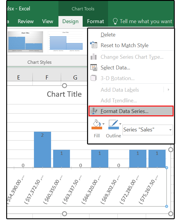
Excel tutorial: Understanding data series This formula is based on the SERIES function, which takes four arguments: =SERIES ( [Series Name], [X Values], [Y Values], [Plot Order]) As I select each series, you can see these arguments change to match the data highlighted on the worksheet. You can edit the SERIES formula if you like. Understanding Excel Chart Data Series, Data Points, and Data Labels Select a data series in a column chart. All columns of the same color are highlighted. Each column is surrounded by a border that includes small dots on the corners. Select the column in the chart to be modified. Only that column is highlighted. Select the Format tab. Stop Excel chart from changing series formatting - Super User edit Solution: As suggested by @ErikF, this page shows how it can be done, i.e., by clicking File > Options > Advanced > Chart > deselect both 'Properties follow chart data point for current workbook' and 'Properties follow chart data point for all new workbooks' microsoft-excel charts formatting Share Improve this question Format data labels for each series in a chart - Stack Overflow Then to add a data label, right click on the data point, and Add Data Label. Then to select a single data label, click on the data label once (this selects all data labels for the series, even if there is only one), and then: 1) click again on the target data label, or 2) press the right arrow, to select the first data label. Then to edit the ...

Dynamically Label Excel Chart Series Lines - My Online Training Hub This formula ensures that the label for the Actual is at the end of the line, and as the data grows the label moves accordingly. Step 3: Select the first label series. Select the outer edge of the chart to expose the contextual Chart Tools ribbon tabs; Select the Format tab (In Excel 2007 & 2010 it's the Layout tab) Click on the drop down Create Dynamic Chart Data Labels with Slicers - Excel Campus Step 6: Setup the Pivot Table and Slicer. The final step is to make the data labels interactive. We do this with a pivot table and slicer. The source data for the pivot table is the Table on the left side in the image below. This table contains the three options for the different data labels. Excel Charts: Dynamic Label positioning of line series - XelPlus To see the label for the Budget series, perform the following: Select your chart and go to the Format tab, click on the drop-down menu at the upper left-hand portion and select Series "Budget". Go to Layout tab, select Data Labels > Right. Right mouse click on the data label displayed on the chart. Select Format Data Labels. Custom Excel Chart Label Positions • My Online Training Hub Custom Excel Chart Label Positions - Setup. The source data table has an extra column for the 'Label' which calculates the maximum of the Actual and Target: The formatting of the Label series is set to 'No fill' and 'No line' making it invisible in the chart, hence the name 'ghost series': The Label Series uses the 'Value ...

How to Make a Sunburst Chart | Documentation 17.0 | Aqua Data Studio

Create a multi-level category chart in Excel - ExtendOffice Double click any series in the chart to open the Format Data Series pane. In the pane, change the Gap Width to 0%. 5. Select the spacing1 data series in the chart, go to the Format Data Series pane to configure as follows. 5.1) Click the Fill & Line icon; 5.2) Select No fill in the Fill section. Then these data bars are hidden. 6.

Working with Charts — XlsxWriter Documentation

Multiple data labels (in separate locations on chart) Re: Multiple data labels (in separate locations on chart) You can do it in a single chart. Create the chart so it has 2 columns of data. At first only the 1 column of data will be displayed. Move that series to the secondary axis. You can now apply different data labels to each series. Attached Files 819208.xlsx‎ (13.8 KB, 265 views) Download

How to Make a Bar Chart in Excel | Smartsheet

How to Rename a Data Series in Microsoft Excel - How-To Geek To do this, right-click your graph or chart and click the "Select Data" option. This will open the "Select Data Source" options window. Your multiple data series will be listed under the "Legend Entries (Series)" column. To begin renaming your data series, select one from the list and then click the "Edit" button.

How to add data labels from different column in an Excel chart?

Prevent Overlapping Data Labels in Excel Charts - Peltier Tech Overlapping Data Labels. Data labels are terribly tedious to apply to slope charts, since these labels have to be positioned to the left of the first point and to the right of the last point of each series. This means the labels have to be tediously selected one by one, even to apply "standard" alignments.

Excel Downloads — improve your graphs, charts and data visualizations — storytelling with data

Separating data into different series for display in a chart - excel ... Shane Devenshire. You could rearrange your data and display it as a stacked column by region: To get the chart you select the range and choose Insert, Column, Stacked Column (second one) Then with the chart selected you choose Chart Tools, Design, Switch Row and Column. If this answer solves your problem, please check Mark as Answered.

Longer Axis Labels in PowerPoint Charts: Why Bar Charts Are Better Than Column Charts?

The first question lots of you might have is So why not using Excel at the first place to load data. How to insert Excels Map Charts. To create a Map Chart in Excel, your data must first be set up correctly. First, you need to have geographical data such as country, state or postcode. You also need some values associated with geographical locations. To insert a Map chart in Excel, select ...

How to create a Lollipop Chart in Excel

Chart's Data Series in Excel - Easy Tutorial 1. Select the chart. Right click, and then click Select Data. The Select Data Source dialog box appears. 2. You can find the three data series (Bears, Dolphins and Whales) on the left and the horizontal axis labels (Jan, Feb, Mar, Apr, May and Jun) on the right. Switch Row/Column

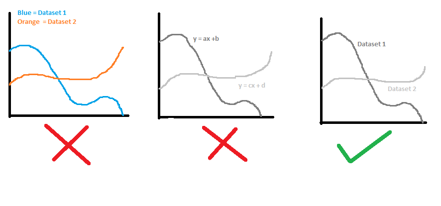
Formatting a graph to label lines with their respective data sets rather than distinguishing ...

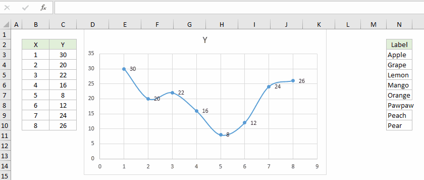
How to Change Excel Chart Data Labels to Custom Values? - Chandoo.org You can change data labels and point them to different cells using this little trick. First add data labels to the chart (Layout Ribbon > Data Labels) Define the new data label values in a bunch of cells, like this: Now, click on any data label. This will select "all" data labels. Now click once again.

Data labels on Excel charts « projectwoman.com

How to Create a Graph with Multiple Lines in Excel Click Select Data button on the Design tab to open the Select Data Source dialog box. Select the series you want to edit, then click Edit to open the Edit Series dialog box. Type the new series label in the Series name: textbox, then click OK.

How to create an Excel chart with no numerical labels? - Super User

How to add data labels from different column in an Excel chart? This method will guide you to manually add a data label from a cell of different column at a time in an Excel chart. 1. Right click the data series in the chart, and select Add Data Labels > Add Data Labels from the context menu to add data labels. 2. Click any data label to select all data labels, and then click the specified data label to select it only in the chart. 3.

Excel charts: add title, customize chart axis, legend and data labels

Formating all data labels in a single series at once. Easiest way to make sure you are doing the right thing is to click off the data labels but on the chart and then right click any data label and choose Format Data Labels. Note the choice on the shortcut menu should not say Format Data Label. What's the difference? the "s" at the end.

Change the format of data labels in a chart You can add a built-in chart field, such as the series or category name, to the data label. But much more powerful is adding a cell reference with explanatory text or a calculated value. Click the data label, right click it, and then click Insert Data Label Field. If you have selected the entire data series, you won't see this command.